By David F Hendry (originally published on VoxEU)

The Industrial Revolution has been of vast benefit to humanity, but it came at the cost of a global explosion in anthropogenic emissions of greenhouse gases. The UK was the first country into the Industrial Revolution. Now it is one of the first countries heading out, with annual CO2 emissions per capita back below the levels of the 1860s. This column presents an econometric model of UK emissions over the last 150 years to establish what has driven them down and reveal the impacts of important policies, especially the Climate Change Act of 2008. Even so, large reductions in all the UK’s CO₂ sources are still required to meet its 2050 target of an 80% reduction from 1970 levels.

The Industrial Revolution began in the UK in the mid-18th century for reasons well explained by Allen (2009). With antecedents in the scientific, technological, and medical knowledge revolutions from two centuries earlier across many countries, the UK was the first country to industrialise on a large scale. The consequences are startling: 250 years later, real income levels per capita are about seven-fold higher (https://ourworldindata.org/economic-growth shows even greater changes in other countries), many killer diseases have been tamed, and longevity has approximately doubled. As Crafts (2002) showed, the average individual would be unwise to swap their life now for that of even one of the richest people several centuries ago; the Industrial Revolution and its successors have been of vast benefit to humanity.

An unintended consequence has been an explosion in atmospheric carbon dioxide and other greenhouse gas emissions. These are by-products of energy production, manufacturing, and transport (all about a quarter of emissions), with agriculture, construction and waste removal creating most of the rest. Although the UK’s first electricity generating power station in 1868 was hydro driven, coal-fired steam-driven power stations were introduced by 1882 and have since produced most of its electricity. The paleo-record over the last 750,000 years of intermittent ice ages shows atmospheric CO₂ levels of between 180 parts per million (ppm) and 300ppm, but these levels now exceed 400ppm. The increases in atmospheric CO₂ recorded since 1958 at Mauna Loa (Sundquist and Keeling 2009) are clearly anthropogenic in origin (e.g. Hendry and Pretis 2013). The climate change induced by increased greenhouse gases has potentially dangerous implications, highlighted by Stern (2006) and recent IPCC reports, leading to the agreement in Paris at COP21 to seek to limit temperature increases to less than 2 Centigrade, and “to pursue efforts to limit it to 1.5C’’.  Much remains to reduce CO₂ emissions towards the net zero level that will be required to stabilize temperatures at any level. Meinshausen et al. (2009) analyse the difficulties of even achieving 2C, but renewable technologies offer hope of at least further large emission reductions.

However, there was a dramatic drop in the UK’s per capita emissions of CO₂ by 2017 to below the levels of the 1860s – the country first into the Industrial Revolution is one of the first out. On 22 April 2017, Britain went a full day without turning on its coal-fired power stations for the first time in more than 130 years, and on 26 May 2017 it generated almost 25% of its electrical energy from solar. The UK’s CO₂ emissions are now just half of their peak level in 1970. How was this reduction achieved?  

UK CO₂ emissions

The data from 1860 on UK CO₂ emissions, fossil fuel volumes, and the ratio of CO₂ emissions to the capital stock are shown in Figure 1. While other greenhouse gas emissions matter, CO₂comprises about 80% of the UK total, with methane, nitrous oxide, and hydrofluorocarbons (HFCs) making up most of the rest in CO₂ equivalents. However, various fossil fuels have different CO2 emissions per unit of energy produced and depend on how efficiently fuels are burnt, from an open fire through vehicles, to a gas-fired power station.

Figure 1a UK CO₂ emissions in millions of tonnes (Mt), 1860 to 2017

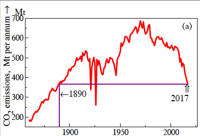
Figure 1b UK coal (Mt), oil (Mt), natural gas (Mt of oil equivalent, Mtoe) and wind+solar (Mtoe), 1860 to 2017

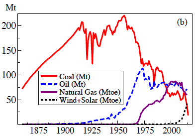
Figure 1c UK CO₂ emissions per capita (tons per annum), 1860 to 2017

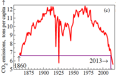
Figure 1d Ratio of UK CO₂ emissions to the capital stock, 1860 to 2017

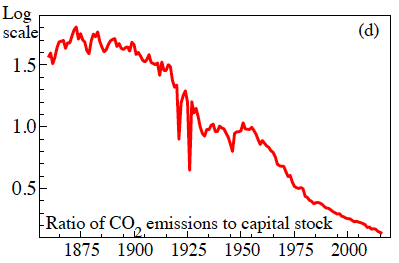
Firgure 1a shows that CO₂ emissions rose strongly from 1860 till about 1916, oscillated violently till about 1946 from the sharp depression at the end of WWI, the General Strike and WWII, and then grew strongly till 1970. After 1984, emissions began to fall slowly, accelerating after 2005 to the end of our time series in 2017, by which time aggregate emissions are below levels first reached in 1890. Figure 1c plots CO₂ emissions per capita, revealing that by 2013 they had fallen below the level at the start of our data period in 1860. Figure 1b records the time series for coal tonnage mined and net oil usage (adding imports to domestic production less exports), natural gas and renewables. Coal output behave similarly to CO₂ emissions till 1956, at which point they turn down and continue falling, dropping well below the tonnage mined in 1860. The sharp dips from miners’ strikes in 1921, 1926 and 1984 are clearly visible. Conversely, oil volumes are essentially zero initially, but rise rapidly after WWII, peak in 1973 with the Oil Crisis, but stabilise from 1981 on, despite a doubling in vehicle travel. Gas usage rises quickly from the late 1960s but has recently fallen slightly: renewables have been growing rapidly this century. Figure 1d plots the log-ratio of CO₂ emissions to the capital stock which started to decline in the 1880s and has dropped by more than 92% since. Since capital embodies the vintage of technology at the time of its construction, tends to be long lasting, and is a key input to production, CO₂ emissions are likely to be strongly affected by the capital stock (e.g. Pfeiffer et al. 2016).

Modelling the changing relationships determining emissions

An obvious feature of the Figure 1 graphs is that all the time series are highly non-stationary. To capture such changing relations, the model includes the two main CO₂ emitters – coal and oil – plus the capital stock and real GDP with dynamics for adjustments to changes in technology, legislation and fuel prices, as well as using impulse indicator saturation (IIS) to detect outliers (from strike action, etc.), and step indicator saturation (SIS) for major permanent shifts (often policy induced). The five climate, fuel, and economic variables form a vector autoregression (VAR), reduced to a viable conditional relationship for CO₂, noting that indicators only capture features not explained by the continuous regressors.

The properties of IIS are analysed by Johansen and Nielsen (2009, 2016); selecting indicators at a tight significance level while retaining variables deemed relevant is described in Hendry and Doornik (2014) where SIS is also investigated (also see Castle et al. 2015). Indicators designed to match known properties, as in using a ν shape for volcanoes, are used in Pretis et al. (2016) as well as for detecting biased forecasts in Ericsson (2017). Here we use Autometrics, a multi-path block search algorithm described in Doornik (2009). An R version is available at https://cran.r-project.org/web/packages/gets/index.html (see Pretis et al. 2018). IIS and SIS add 307 indicators to the nine conditional regressors but selecting at 0.1% would retain 0.3 of an indicator on average by chance. In total, 11 indicators were retained when estimating over 186−2011, entailing 4 location shifts. Three of these were identifiable with major events. We did not impose that policy had an effect – the data tell us it did as follows:

• in 1926, when an Act of Parliament created the UK’s nationwide electricity grid;
• in 1969, at the start of nationwide conversion from coal gas to natural gas;
• in 2010, following implementation of the UK’s Climate Change Act of 2008 and the EU’s renewables directive of 2009.

We also found a step in 1991 which revealed that emissions were higher later than the model otherwise explains. There were also five impulse or blip indicators for outliers. Next, selecting from the nine regressors, keeping significant indicators, eliminated only current dated GDP. Third, the null hypothesis of no cointegration is strongly rejected, leading to the solved long-run equilibrium-correction (EqCM) relation that we use.¹

Autometrics step indicators, denoted S_19xx, end at the dates shown, so reflect levels before those dates (2010 is excluded here as at the sample end). The long-run negative effect of GDP possibly reflects the move from manufacturing to a service-based economy, with the fossil fuel coefficients close to, but somewhat above, their carbon contents, with a major role for the capital stock. Finally, the relationship was transformed to a non-integrated representation in terms of differences and the lagged EqCM. Changes in oil, coal and the capital stock all lead to changes in emissions, which then equilibrates back to the long-run EqCM relation. There are very large perturbations from this relationship, involving step shifts and impulses. Figure 2 records the outcome mapped back to levels (as otherwise the massive outliers dominate a graph of the changes).

Figure 2 Fitted and actual values for UK CO2 emissions

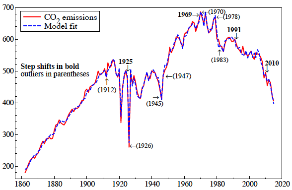
Note: Step shifts are shown in bold, outliers in parentheses.

System unconditional forecasts

To check the constancy of the model after 2011, Figure 3 records 1 through four-steps ahead dynamic forecasts of emissions from the unconditional VAR with and without having selected by SIS.

Figure 3 Dynamic forecasts from the VAR with and without having selected by SIS

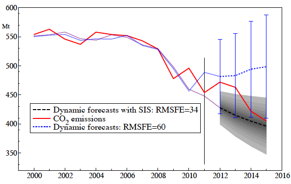
As can be seen, the SIS-based forecasts are considerably more accurate, and have a root mean square forecast error (RMSFE) that is almost half of that without.

Testing the UK’s achievement of its 2008 Climate Change Act targets for CO₂

The Act’s five-year targets were translated into annual magnitudes, starting 20Mt above and ending 20Mt below the average for the period, scaled by 0.8 as the share of CO₂ in UK greenhouse gas emissions. A decade has elapsed since the Act, so there are ten annual observations on CO₂emissions to compare to the targets, from which we calculated a test of the difference between targets and outcomes being zero, starting in 2009 as the Act could not have greatly influenced the emissions in its year of implementation. A graph is shown in Figure 4. The null of “emissions=targets” is strongly rejected on the negative side with a mean of −18Mt. The budget for 2018–2022 of 2544 Mt, roughly 410 Mt per annum of CO₂, is undemanding given the 2017 level of 368 Mt, but should not induce complacency as the easiest reductions have been accomplished with coal use now almost negligible.

Conclusions

Having been first into the Industrial Revolution that transformed the world’s wealth at the cost of climate change, the UK is one of the first out in terms of its reduced CO₂ emissions, which have dropped below the level first reached in 1890. In per capita terms, CO₂ emissions are now just 53% of the level 1890 and below that of 1860 – when the UK was the ‘workshop of the world’ – despite per capita real incomes being more than seven-fold higher. This has been achieved mainly by driving coal out of energy production and expanding GDP without increases in other fuels.

The model presented here explains CO₂ emissions data over 1860–2015 in terms of coal and oil usage, capital stock and GDP, taking account of their non-stationary nature, with many turbulent periods and major shifts over the 155 years. GDP had a negative effect given the other explanatory variables, probably reflecting an increased share of services, notwithstanding which, the model entails a non-linear ‘environmental Kuznets curve’ between emissions and GDP. Improvements in multi-step forecasts highlighted the advantages of taking account of in-sample outliers and shifts using impulse and step indicator saturation, despite those creating more candidate variables to select over than observations.

Figure 4a Five-year targets for CO₂

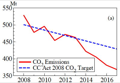
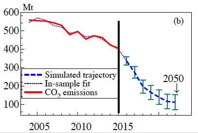
Figure 4b Reductions in CO₂ emissions from model simulation: no coal, 75% reductions in oil and gas; 50% reductions from agriculture, construction and waste emissions, compressed to five-year intervals after 2015

The policy implications are that:

• climate policy can be effective;
• reducing CO₂emissions has not had a large cost at the aggregate level, but local losses need to be addressed;
• the UK’s targets of an 80% reduction from the 1990 baseline of 590 Mt are only achievable with major reductions in all emissions sources; and
• even greater CO₂emissions reduction efforts, or increased re-absorption, are needed to achieve a net zero emissions goal.

Already, onshore wind is its cheapest power-generating technology, and while natural gas combined cycle gas turbines seem competitive, they cease to be so if carbon capture and storage is mandated, in which setting solar large-scale PV is second cheapest. Both wind and solar can benefit from further returns to scale but suffer from good storage systems. Although the UK ‘imports’ a substantial amount of embedded carbon, that will reduce as other countries move to implement reduced emissions.

References

Allen, R C (2009), The British Industrial Revolution in Global Perspective, Cambridge University Press.

Castle, J L, J A Doornik and D F Hendry (2012), “Model selection when there are multiple breaks”, Journal of Econometrics 169: 239–246.

Crafts, N F R (2002), “Is economic growth good for us?”, public lecture, Royal Economic Society.

Doornik, J A (2009), “Autometrics”, in J L Castle and N Shephard (eds), The Methodology and Practice of Econometrics, Oxford University Press, pp. 88–121.

Ericsson, N R (2017), “How biased are U.S. Government forecasts of the Federal Debt?”,International Journal of Forecasting 33: 543–559.

Hendry, D F (2018), “First-in, First-out: Modelling the UK’s CO2 Emissions, 1860–2016”, Working Paper, Nuffield College, University of Oxford.

Hendry, D F and J A Doornik (2014), Empirical Model Discovery and Theory Evaluation, MIT Press.

Hendry, D F and F Pretis (2013), “Anthropogenic influences on atmospheric CO2”, in R Fouquet (ed.), Handbook on Energy and Climate Change, Edward Elgar, pp. 287–326.

Hendry, D F and F Pretis (2016), “All Change! Non-stationarity and its implications for empirical modelling, forecasting and policy”, Oxford Martin School Policy Paper.

Johansen, S and B Nielsen (2009), “An analysis of the indicator saturation estimator as a robust regression estimator”, in J L Castle and N Shephard (eds), The Methodology and Practice of Econometrics, Oxford University Press, pp. 1–36.

Johansen, S and B Nielsen (2016), “Asymptotic Theory of Outlier Detection Algorithms for Linear Time Series Regression Models”, Scandinavian Journal of Statistics 43: 321–348.

Meinshausen, M et al. (2009), “Greenhouse-gas emission targets for limiting global warming to 2◦C”, Nature 458: 1158–1162.

Pfeiffer, A, R Millar, C Hepburn and E Beinhocker (2016), “The ‘2◦C capital stock’ for electricity generation: Committed cumulative carbon emissions from the electricity generation sector and the transition to a green economy”, Applied Energy 179: 1395–1408.

Pretis, F, L Schneider, J E Smerdon and D F Hendry (2016), “Detecting volcanic eruptions in temperature reconstructions by designed break-indicator saturation”, Journal of Economic Surveys 30: 403–429.

Stern, N (2006), The Economics of Climate Change:  The Stern Review, Cambridge University Press.

Endnotes

[1] Letting S(date) denote the date the step shifts end, the exact formula is: Emissions = 2.7Coal + 2.1Oil + 0.2Capital − 8.2GDP + 42S(1925) − 72S(1969) −  43S(1991)